|
1
|
- Hilbert Space
- H2 and H¥ Functions
- State Space Computation of H2 and H¥ norms
|
|
2
|
- Inner Product: Let V be a vector
space over C. An inner product on V is a complex valued function, <·, ·>: V ´ V ® C
- Such that for any x, y, z ÎV and a, bÎC
- (i) <x, ay+bz>=a<x,y>+b<x,z>
- (ii) <x,y>=<y,z>* (complex conjugate)
- (iii) <x,x> >0 if x¹ 0.
- Inner product on Cn:
- x and y are orthogonal if Ð (x,y)= ½p
|
|
3
|
- A vector space V with an inner product is called an inner product
space.
- Inner product induced norm ||x||
:= Ö<x,x>
- Distance between vectors x and y : d(x,y) = ||x - y|| .
- Two vectors x and y are orthogonal if <x,y> = 0, denoted x ^ y.
- Properties of Inner Product:
- |<x, y>|£||x|| ||y|| (Cauchy-Schwarz inequality).
Equality holds iff x=ay for some constant a or y=0.
- ||x+y||2+||x-y||2=2||x||2+2||y||2
(Parallelogram law)
- ||x+y||2=||x||2+||y||2 if x ^ y.
|
|
4
|
- Hilbert Space: a complete inner product space. (We shall not discuss the
completeness here.)
- Examples:
- Cn with the usual
inner product.
- Cn ×m with the following inner product
- <A, B> := Trace A*B
" A,
B Î Cn
×m
- L2[a,b]: all square integrable and Lebesgue measurable
functions defined on an interval [a,b] with the inner product
- <f, g> := aòb f(t)*g(t)dt, Matrix form: <f, g> := aòb Trace[
f(t)*g(t)]dt.
- L2 = L2 (-¥, ¥): <f, g> := - ¥ ò¥ Trace[
f(t)*g(t)]dt.
- L2+ = L2[0, ¥): subspace of L2(-¥, ¥).
- L2- = L2(-¥, 0]: subspace of L2(-¥, ¥).
|
|
5
|
- Let S Ì C be an
open set, and let f(s) be a complex valued function defined on S, f(s) : S ® C. Then f(s)
is analytic at a point z0 in S if it differentiable at z0
and also at each point in some
neighborhood of z0.
- It is a fact that if f(s) is
analytic at z0 then f has continuous derivatives of all
orders at z0. Hence, it has a power series representation at z0.
- A function f(s) is said to be
analytic in S if it has a derivative or is analytic at each point of S.
- Maximum Modulus Theorem: If f(s) is defined and continuous on a
closed-bounded set S and analytic on the interior of S, then
- maxsÎS êf(s) ê= maxsζS êf(s) ê
- where ¶S denotes the boundary of S.
|
|
6
|
- L2(jR) Space: all complex matrix functions F such that the
integral below is bounded:
- with the inner product
- and the inner product induced norm is given by
- RL2(jR) or simply RL2: all real rational strictly
proper transfer matrices with no poles on the imaginary axis.
|
|
7
|
- H2 Space: a (closed) subspace of L2(jR) with
functions F(s) analytic in Re(s) > 0.
- RH2 (real rational subspace of H2 ): all strictly
proper and real rational stable transfer matrices.
- H2^ Space: the orthogonal complement of H2
in L2, i.e., the (closed) subspace of functions in L2
that are analytic in Re(s)<0.
- RH2^ ( the real rational subspace of H2^ ): all
strictly proper rational antistable transfer matrices.
- Parseval’s relations: (between time domain and frequency domain)
|
|
8
|
- L¥
(jR) Space: L¥ (jR)
or simply L¥ is a Banach space of matrix-valued (or
scalar-valued) functions that are (essentially) bounded on jR, with norm
- RL¥
(jR) or simply RL¥: all proper and real rational transfer matrices
with no poles on the imaginary axis.
- H¥
Space: H¥ is a (closed) subspace of L¥ with
functions that are analytic and bounded in the open right-half plane.
The H¥ norm is defined as
- The second equality can be regarded as a generalization of the maximum
modulus theorem for matrix functions. See Boyd and Desoer [1985] for a
proof.
- RH¥:
all proper and real rational stable transfer matrices.
|
|
9
|
- H¥-
Space: H¥- is a (closed) subspace of L¥ with
functions that are analytic and bounded in the open left-half plane. The
H¥- norm is defined as
- RH¥-
: all proper real rational antistable transfer matrices.
- Examples: H2 functions: 1/s+1, e-hs/s+2, …
- H¥
functions: 5, 1/s+1, 5s+1/s+2, e-hs/s+2, 1/s+1+0.1e-hs,
…
- L¥
functions: 5, 1/s+1,1/(s+1)(s-2), 1/s-1+0.1e-hs, …
|
|
10
|
- Let G(s) be a p× q transfer matrix. Then a multiplication operator is
defined as MG:
L2 ® L2 , MG f=Gf
- Then
- Proof: It is clear that ||G||¥ is the upper bound:
- To show that ||G||¥ is the least upper bound, first choose
a frequency w0
where is maximum,
i.e.,
|
|
11
|
- and denote the singular value decomposition of G(jw0) by
- where r is the rank of G(jw0) and ui ,vi
have unit length.
- If w0<
¥, write v1(jw0) as
- where aiÎR is such that qiÎ(-p,0]. Now let 0 £ bi £ ¥ be such that
- (with bi=¥ if qi=0 ) and let f
be given by
|
|
12
|
- (with 1 replacing if qi=0) where a
scalar function is chosen so that
- where e is a
small positive number and c is chosen so that has unit 2-norm, i.e., This in turn implies
that f has unit 2-norm.
- Similarly, if w0=
¥, the
conclusion follows by letting w0® ¥ in the above.
|
|
13
|
- Let G(s) Î L2
and g(t) = L-1 [G(s)]. Then
- Consider G(s)=C(sI-A)-1B Î RH2 . Then we have
- ||G(s)||22=
trace(B*L0B) = trace(CLcC*)
- where L0 and Lc
are observability and controllability Gramians:
- ALc+LcA*+BB* = 0 A*L0+L0A+C*C
= 0.
|
|
14
|
- Proof: Note that g(t) = L-1 [G(s)]=CeAtB, t ³0, and
- Then
|
|
15
|
- Hypothetical input-output experiments:
- Apply the impulsive input d(t)ei (d(t) is the unit impulse and ei is the ith
standard basis vector) and denote the output by zi (t)( =
g(t)ei ). Then ziÎ L2+ ( assuming D = 0) and
- Can be used for nonlinear time varying systems.
|
|
16
|
- Example: Consider a transfer
matrix
- with
- Then the command h2norm(Gs) gives ||Gs||2=
0.6055 and h2norm(cjt(Gu)) gives ||Gu||2=
3.182. Hence
- >> P = gram(A,B); Q = gram(A´,C´); or P = lyap(A,B*B´);
- >> [Gs,Gu] = sdecomp(G); % decompose into stable and antistable parts.
|
|
17
|
- Rational Functions: Let G(s) Î RL¥ :
- the farthest distance the Nyquist plot of G from the origin
- the peak on the Bode magnitude plot
- estimation: set up a fine grid of frequency points, {w1,…, wN}.
|
|
18
|
- Characterization: Let g > 0
and Then
- where
- and R =g 2I-D*D.
- Proof: Let F(s) =g 2I-G~(s)G(s).
- Then ||G||¥ < g Û F(jw)>0, " wÎ R È {¥}Û detF(jw)¹ 0, " wÎ R since F(¥)=R>0 and F(jw) is continuous. Û F(s) has no imaginary
axis zero. Û F -1(s) has no imaginary axis pole.
- Û H has no jw axis eigenvalues if the above realization has
neither uncontrollable modes nor unobservable modes on the imaginary
axis.
|
|
19
|
- We now show that the above realization for F -1(s) indeed has neither
uncontrollable modes nor unobservable modes on the imaginary axis.
- Assume that jw0 is an eigenvalue of H but not a pole
of F -1(s).
Then jw0
must be either an unobservable mode of ([R-1D*C R-1B*], H) or an
uncontrollable mode of (H, ). Suppose jw0 is an
unobservable mode of
- ([R-1D*C R-1B*], H). Then there
exists an
such that
- Hx0 = jw0 x0 ,
[R-1D*C R-1B*]x0=
0. Û
- (jw0 I-A*)x1=0, (jw0 I+A*)x2=-C*Cx1, D*Cx1+B*x2=0.
- Since A has no imaginary axis eigenvalues, we have x1 = 0
and x2 = 0. Contradiction!!!
- Similarly, a contradiction will also be arrived if jw0 is assumed to be an uncontrollable
mode of (H, ).
|
|
20
|
- (a) select an upper bound gu and a lower bound gl such that
- gl £ ||G||¥ £ gu
- (b) if (gu-gl)/gl £ specified level, stop; ||G||¥ » (gu+gl)/2.
Otherwise go to next step.
- (c) set g = (gl + gu) /2;
- (d) test if ||G||¥ < g by calculating the eigenvalues of H
with this g;
- (e) if H has an eigenvalue on jR set gl = g ; otherwise set gu = g ; go back to step (b).
- In all the subsequent discussions, WLOG we can assume g = 1 by a
suitable scaling since ||G||¥ < g Û || g -1G||¥ <1.
|
|
21
|
- Estimating the H¥ norm experimentally: the maximum magnitude of
the steady-state response to all possible unit amplitude sinusoidal
input signals.
- z(t)=|G(j w)|sin(wt+ÐG(j w)) u(t)=sin wt
- Let the sinusoidal input u(t) as shown below. Then the steady-state response of the
system can be written as
- for some yi, i, i= 1,2,….,p, and furthermore,
- where ||•|| is the Euclidean norm.
|
|
22
|
- Consider a mass/spring/damper system as shown in Figure 4.2.
- The dynamical system can be described by the following differential
equations:
|
|
23
|
- Suppose that G(s) is the transfer matrix from (F1 , F2)
to (x1 , x2); that is,
- and suppose k1=1, k2 =4, b1 =0.2, b2
= 0.1, m1 =1, and m2=2 with appropriate units.
- >>G=pck(A,B,C,D);
- >>hinfnorm(G,0.0001) or linfnorm(G,0.0001) % relative error £0.0001
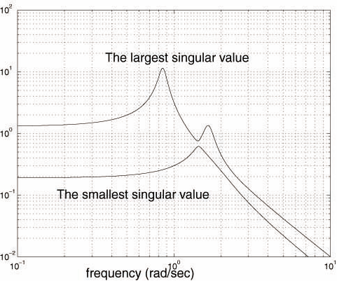
- >>w=logspace(-1,1,200);
%200 points between 0.1=10-1 and 10=101;
- >>Gf=frsp(G,w); %computing frequency response;
- >>[u,s,v]=vsvd(Gf); %SVD at each frequency;
- >>vplot(‘liv,lm’,s), grid
%plot both singular values and grid.
- ||G||¥
=11.47=the peak of the largest singular value Bode plot in Figure
4.3.
|
|
24
|
|
|
25
|
- Since the peak is achieved at w max = 0.8483, exciting the system
using the following sinusoidal input
- gives the steady-state response of the system as
- This shows that the system response will be amplified 11.47 times for
an input signal at the frequency wmax, which could be undesirable if F1
and F2 are disturbance force and x1 and x2
are the positions to be kept steady.
|
|
26
|
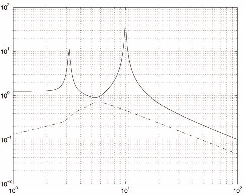
- Example 2: Consider a two-by-two transfer matrix
- A state-space realization of G can be obtained by using the following
MATLAB commands:
- >>G11=nd2sys([10,10],[1,0.2,100]);
- >>G12=nd2sys(1,[1,1]);
- >>G21=nd2sys([1,2],[1,0.1,10]);
- >>G22=nd2sys([5,5],[1,5,6]);
- >>G=sbs(abv(G11,G21),abv(G12,G22));
- Next, we setup a frequency grid to compute the frequency response of G
and the singular values of G(jw) over a suitable range of frequency.
- >>w = logspace(0,2,200); %
200 points between 1=100 and 100=102;
- >>Gf=frsp(G,w); % computing frequency response;
|
|
27
|
- >>[u,s,v]=vsvd(Gf); % SVD
at each frequency;
- >>vplot(‘liv,lm’,s), grid %plot both singular values and grid;
- >>pkvnorm(s) % find the norm from the frequency response of the
singular values.
- The singular values of G(j w) are plotted in Figure 4.4, which gives an
estimate of ||G||¥ »32.861. The state-space bisection algorithm
described previously leads to ||G||¥ = 50.25±0.01 and the corresponding MATLAB command is
- >>hinfnorm(G,0.0001) or linfnorm(G,0.0001) % relative error £0.0001.
- The preceding computational results show clearly that the graphical
method can lead to a wrong answer for a lightly damped system if the
frequency grid is not sufficiently dense. Indeed, we would get ||G||¥ » 43.525,
48.286 and 49.737 from the graphical method if 400,800, and 1600
frequency points are used respectively.
|
|
28
|
|

 Notes
Notes