|
1
|
- Robust stabilization of Coprime factors
- Robust Stabilization of Normalized Coprime Factors
- H¥ Loop
Shaping Design
- Weighted H¥ Control Interpretation
- Optimal Stability Margin
- Further Guidelines for Loop Shaping
|
|
2
|
|
|
3
|
|
|
4
|
|
|
5
|
|
|
6
|
|
|
7
|
|
|
8
|
|
|
9
|
- Given nominal model P(s).
- (1) Loop Shaping: Obtain a desired open-loop shape (singular values) by
using a precompensator W1 and/or a postcompensator W2,
- Ps=W2PW1
- Assume that W1 and W2 are such that Ps
contains no hidden modes.
- (2) (a) Calculate robust stability margin bopt(Ps).
If bopt(Ps) <<1, return to (1) and adjust W1
and W2 . (b) Select e £ bopt(Ps)
, then synthesize a stabilizing controller K¥ which satisfies
- (3) The final controller K=W1K¥W2
|
|
10
|
- A typical design works as follows: the designer inspects the open-loop
singular values of the nominal plant, and shapes these by pre- and/or
postcompensation until nominal performance (and possibly robust
stability) specifications are met. (Recall that the open-loop shape is
related to closed-loop objectives.) A feedback controller K¥ with
associated stability margin (for the shaped plant) e £ bopt(Ps)
is then synthesized. If bopt(Ps) is small, then
the specified loop shape is incompatible with robust stability
requirements, and should be adjusted accordingly, then K¥ is
reevaluated.
- Note that the final controller is K=W1K¥W2 , so it is necessary to check if
the loop properties are significantly changed. It is helpful to choose W1
and W2 with small condition numbers.
- Only W1 or W2 is needed if P is SISO.
|
|
11
|
|
|
12
|
|
|
13
|
|
|
14
|
- >> bp,k = emargin (P,K); % given P and K, compute bP,K
- >> [Kopt, bp,k ]=ncfsyn(P,1); % find the
optimal controller Kopt.
- >> [Ksub, bp,k ] = ncfsyn(P,2); % find a
suboptimal controller Ksub.
|
|
15
|
- Let P = NM-1 be normalized right coprime factorization. Then
- small l(P) Þ small bopt(P)
- Let the open right-half plane zeros and poles of P be:
- z1, z2,…,
zm, p1, p2,…,
pk
- Define
- Then P(s)=P0(s)Nz(s)/Np(s)
- where P0(s) has no open right-half plane zeros and poles.
|
|
16
|
- Let N0(s) and M0(s) be stable and minimum phase
spectral factors:
- Then P0= N0 / M0 is a normalized coprime factorization
and (N0 Nz) and (M0 Np) form
a pair of normalized coprime factorizations of P.
- Thus
- where r>0, -p/2<q< p/2, and
|
|
17
|
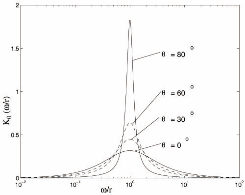
- Kq(w/r) large near w=r: |N0(rejq)| will be
small if |P(jw)| is
small near w=r
and |M0(rejq)| will be small if |P(jw)| is large near w=r.
- Large q: Kq(w/r) very large near w=r and small otherwise. Hence |N0(rejq)| and |M0(rejq)| will
essentially be determined by |P(jw)| in a very narrow frequency range near w=r when q is large.
- On the other hand, when q is small, a larger range of frequency response |P(jw)| around w=r will have affect on
the value |N0(rejq)| and |M0(rejq)|(This, in
fact, will imply that a right-plane zero (pole) with a much larger real
part than the imaginary part will have much worse effect on the
performance than a right-plane zero (pole) with a much larger imaginary
part than the real part).
|
|
18
|
- Recall (bopt(P))
2 £|N0(s)Nz(s)|2
+|M0(s)Np(s)|2 " Re(s)>0
- Let s=rejq and note that Nz(zi)=0 and
Np(pj)=0. Then the bound can be small if
- |Nz(s)| and |Np(s)| are both small for some s.
That is, |Nz(s)|»0 (i.e., s is close to a right-half plane zero of
P) and |Np(s)|»0 (i.e., s is close to a right-half plane pole of
P).
- This is possible if P(s) has a right-half plane zero near a right-half
plane pole. (See Example 16.1.)
- |Nz(s)| and |M0(s)| are both small for some s.
That is, |Nz(s)|»0 (i.e., s
is close to a right-half plane zero of P) and |M0(s)|»0 (i.e., |P(jw)| is large around w=|s|=r ).
- This is possible if |P(jw)| is large around w=r where r is the modulus of a right-half plane
zero of P (See Example16.2)
|
|
19
|
- |Np(s)| and |N0(s)| are both small for some s.
That is, |Np(s)|»0 (i.e., s is close to a right-half plane pole of
P) and |N0(s)|»0 (i.e., |P(jw)| is small around w=|s|=r).
- This is possible if |P(jw)| is small around w=r where r is the modulus of a right-half plane
pole of P (See Example 16.3)
- |N0(s)| and |M0(s)| are both small for some s.
That is, |N0(s)|»0 (i.e., |P(jw)| is small around w=|s|=r) and |M0(s)|»0 (i.e., |P(jw)| is large around w=|s|=r).
- The only way in which |P(jw)| can be both small and large at frequencies
near w=r is
that |P(jw)|
is approximately equal to 1 and the absolute value of the slope of |P(jw)| is large. (See
Example 16.4)
|
|
20
|
- Example 16.1
- bopt(P1)
will be very small for all K whenever r is close to 1 (i.e.,
whenever there is an unstable pole close to an unstable zero).
|
|
21
|
|
|
22
|
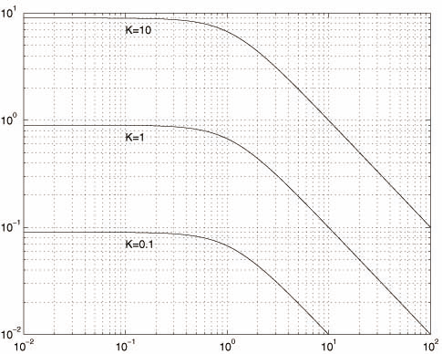
- Example 16.2
- bopt(P2) will be small if |P2(jw)| is
large around w =1, the modulus of the right-half plane zero.
- Note that bopt(L/s) = 0.707 for any L and bopt(P2)® 0.707 as K ® 0. This
is because |P2(jw)| around the frequency of the right-half plane
zero is very small as K ® 0.
|
|
23
|
|
|
24
|
- bopt(P3) will be small if |P3(jw)| is large around the
frequency of w=1 (the modulus of the right-half plane zero).
- For zeros with the same modulus, bopt(P3)
will be smaller for a plant with relatively larger real part zeros than
for a plant with relatively larger imaginary part zeros (i.e., a pair of
real right-half plane zeros has a much worse effect on the performance
than a pair of almost pure imaginary axis right-half plane zeros of the
same modulus).
|
|
25
|
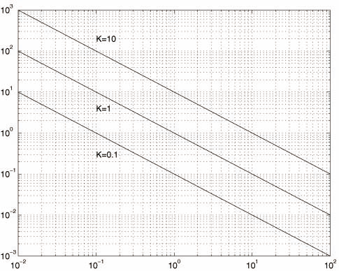
- Example 16.3
- bopt(P4) will be small if |P4(jw)| is small around the
frequency of w=1 (the modulus of the right-half plane pole).
- Note that bopt(P4)® 0.707
as K ® ¥. This is because |P4(jw)| is very large around
the the frequency of the modulus of the right-half plane pole as K ® ¥.
|
|
26
|
|
|
27
|
- bopt(P5) will be small if |P5(jw)| is small around the
frequency of the modulus of the right-half plane pole.
- For poles with the same modulus, bopt(P5) will be
smaller for a plant with relatively larger real part poles than for a
plant with relatively larger imaginary part poles(i.e., a pair of real
right-half plane poles has a much worse effect on the performance than a
pair of almost pure imaginary axis right-half plane poles of the same
modulus).
|
|
28
|
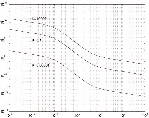
- Example 16.4
- K = 10-5 : slope near
crossover is not too large Þ bopt(P6)
not too small.
- K = 104 : Similar.
- K = 0.1: slope near crossover is
quite large Þ bopt(P6) quite small.
|
|
29
|
- Based on the preceding discussion, we can give some guidelines for the
loop-shaping design.
- The loop transfer function should be shaped in such a way that it has
low gain around the frequency of the modulus of any right-half plane
zero z. Typically, it requires that the crossover frequency be much
smaller than the modulus of the right-half plane zero; say, wc<|z|/2
for any real zero and wc <|z| for any complex zero with a
much larger imaginary part than the real part (see Figure 16.6).
- The loop transfer function should have a large gain around the frequency
of the modulus of any right-half plane pole.
- The loop transfer function should not have a large slope near the crossover
frequencies.
- These guidelines are consistent with the rules used in classical
control theory (see Bode[1945] and Horowitz[1963]).
|

 Notes
Notes