1	Chapter 10: m and m-Synthesis general framework analysis and synthesis methods for unstructured uncertainty stability with structured uncertainties unstructured perturbation structured perturbation definition of SSV examples tighter bounds tightness of bounds computing bounds using Matlab structured robust stability structured robust stability theorem robust performance extension to nonlinear time varying uncertainties HIMAT example skewed problem overview on m-synthesis
2	General Framework Every problem can be put in the general framework with For analysis, the controller can be absorbed into the system:
3	Analysis and Synthesis Methods for Unstructured Uncertainty
4	Stability with Structured Uncertainties Assume D(s)=diag[d₁I_r1, …, d_sI_rs, D₁, …, D_F] Î RH_¥ with \|\|d_i\|\|_¥<1 and \|\|D_j\|\|_¥<1. Robust Stability Û The interconnection is stable. Stability Conditions: (1) (sufficient condition) \|\|M₁₁\|\|_¥£1 Conservative: ignoring structure of D(s). (2) (necessary conditions ) Test for each d_i(D_j) individually (assuming no uncertainty in other channels): \|\|(M₁₁)_ii\|\|_¥£1 Optimistic: ignoring interaction between the d_i(D_j).
5	Unstructured Perturbation Problem: Given M Î C ^p^´^q , find a smallest D Î C ^p^´^q (no structure imposed on D) in the sense of such that det(I-MD)=0. It is easy to see that with a smallest “destabilizing” So the largest singular value of M can be defined as
6	Structured Perturbation Problem: Given M Î C ^p^´^q , find a smallest D Î D D={diag[d₁I_r1, …, d_sI_rs, D₁, …, D_F] Î C ^p^´^q : d_i Î C, D_jÎ C ^m^j^´^m^j } such that det(I-MD)=0. We shall call 1/a_min as structured singular value (SSV).
7	Definition of SSV For M Î C ⁿ^´ⁿ , m_D(M) is defined as unless no D Î D makes I-MD singular, in which case m_D(M) :=0. If D={dI_n : d Î C} (S=1, F=0, r₁=n), then m_D(M)=r(M), the spectral radius of M. If D={D Î C ⁿ^´ⁿ} (S=0, F=1, m₁=n), then m_D(M) = . Thus we have the following bounds: r(M) £ m_D(M) £
8	Examples Let D={diag[d₁, d₂] Î C ²^´² : d_i Î C}. Consider two matrices: Thus neither r(M) nor provides useful bounds even in these simple cases
9	Tighter Bounds To obtain tighter bounds, define U={U Î D : UU*=I_n}
10	Tightness of Bounds
11	Computing Bounds Using Matlab Example: Let M be a 13x13 matrix and suppose D is given by where the size of D is specified by the matrix blk. >> [bounds,rowd] = mu(M,blk) >> [D_l,D_r] = unwrapd(rowd,blk)
12	Structured Robust Stability We are interested in the following question: How large D (in the sense of \|\|D\|\|_¥) can be without destabilizing the feedback system? Since the closed-loop poles are given by det(I-G(s)D)=0 the feedback system becomes unstable if det(I-G(s)D(s))=0 for some s in the closed right half plane. Now let a>0 be a sufficiently small number such that the closed-loop system is stable for all stable \|\|D\|\|_¥< a. Next increase a until a_max so that the closed-loop system becomes unstable. So a_max is the robust stability margin. Consider a general feedback interconnection where D is structured uncertainty block and G(s) is the interconnection matrix.
13	Structured Robust Stability Theorem Define D :={D(·) Î RH_¥ : D(s₀) Î D for all s₀Î } Theorem: Let b>0. The interconnected system is well-posed and internally stable for all D(·) Î D with \|\|D\|\|_¥< 1/b if and only if
14	Robust Performance Let Theorem: Let b>0. For all D(s) Î D with \|\|D\|\|_¥< 1/b , the system is well-posed, internally stable, and \|\|F_u(G_p, D) \|\|_¥£ b if and only if
15	Extension to Nonlinear Time Varying Uncertainty Suppose D Î D_N is a structured Nonlinear (Time-varying) Uncertainty and suppose D is constant scaling matrix such that DDD^-1 Î D_N. (Note that we do not require DD=DD.) Then a sufficient stability condition for all D Î D_N with \|\|D\|\|_¥< 1, is (by small gain theorem) \|\|D^-1G(s)D\|\|_¥£ 1
16	HIMAT Example We shall first find a H_¥ controller using Matlab (details will be discussed in later chapters. Just follow the steps here.), which gives g=1.8612= \|\|G_p\|\|_¥ , a stabilizing controller K, and a closed loop transfer matrix G_p:
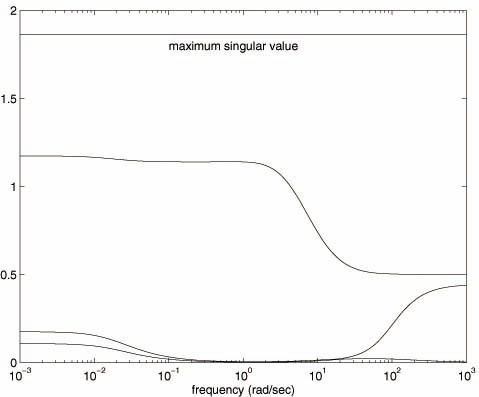
17	"Now generate the singular value..." Now generate the singular value frequency responses of G_p: >> w = logspace(-3,3,300); >> Gpf = frsp(G_p,w); % Gpf is the frequency response of G_p; >> [u,s,v] = vsvd(Gpf); >> vplot(‘liv, m’, s) The singular value frequency responses of G_p are shown in Figure 10.6
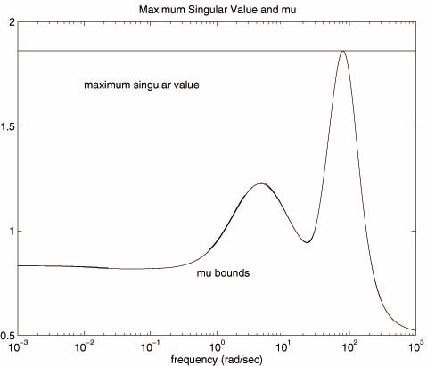
18	"To test the robust stability" To test the robust stability, we need to compute \|\|G_p11\|\|_¥ , >> G_p11 = sel(G_p, 1:2, 1:2); >> norm_of_G_p11 = hinfnorm(G_p11,0.001); which gives \|\|G_p11\|\|_¥ =0.933<1. So the system is robustly stable. To check the robust performance, we shall compute the for each frequency with >> blk = [2,2;4,2]; >> [bnds,dvec,sens,pvec] = mu(Gpf,blk); >> vplot(‘liv,m’,vnorm(Gpf),bnds) >> title(‘Maximum Singular Value and mu’) >> xlabel(‘frequency(rad/sec)’) >> text(0.01,1.7,’maximum singular value’) >> text(0.5,0.8,’mu bounds’)
19	"The structured singular value" The structured singular value are shown in Figure 10.7. It is clear that the robust performance is not satisfied. Note that Using a bisection algorithm, we can also find the worst performance:
20	Skewed Problem Recall the skewed problem in Chapter 8. It can be shown that robust performance problem is equivalent to a 2 block structure singular value with the following interconnection matrix So the robust performance condition is for all w³0.
21	"Now assume W_e=w_sI," Now assume W_e=w_sI, W_d=I, W₁=I, W₂=w_tI and P is stable and has a stable inverse (I.e., minimum phase) and K(s)=P^-1(s)l(s) such that K(s) is proper and the closed-loop is stable. Then S_o=S_i=1/(1+l(s))I=e(s)I, T_o=T_i=l(s)/(1+l(s))I=t(s)I and Let the SVD of P(jw) be P(jw)=USV*, S = diag(s₁, s₂ , …, s_m) with and where m is the dimension of P. Then
22	"Note that" Note that where P₁ and P₂ are permutation matrices. Hence
23	"The maximum is achieved at" The maximum is achieved at and Conclusion: The structure singular value of the skewed problem is (approximately) proportional to the square root of the condition number of the plant.
24	Overview on m Synthesis Consider a general feedback system with interconnection G. Find a stabilizing controller K so that the following m-norm is minimized: This problem is called m-synthesis. The m-synthesis is not yet fully solved. But a reasonable approach is to “solve” by iteratively solving for K and D, i.e., first minimizing over K with D fixed, then minimizing point-wise over D with K fixed, then again over K, and again over D, etc. This is the so-called D-K Iteration.
25	"Fix D" Fix D is a standard H_¥ optimization problem. Fix K is a standard convex optimization problem and it can be solved point-wise in the frequency domain: Note that when S = 0, (no scalar blocks)
26	"Details of D-K Iterations:" Details of D-K Iterations: (i) Fix an initial estimate of the scaling matrix D_w Î D point-wise across frequency. (ii) Find scalar transfer functions d_i(s), d_i^-1(s) Î RH_¥ for i =1,…, (F-1) such that \|d_i(jw)\|» d_i^w . (iii) Let D(s)=diag(d₁(s)I, …, d_F-1(s)I, I). Construct a state space model for system (iv) Solve an H_¥ optimization problem to minimize over all stabilizing K’s. Denote the minimizing controller by
27	"(v)" (v) Minimize over D_w Î D point-wise across frequency. The minimization itself produces a new scaling function . (vi) Compare with the previous estimate D_w, Stop if they are close, otherwise, replace D_w with and return to step (ii). The joint optimization of D and K is not convex and the global convergence is not guaranteed, many designs have shown that this approach works well.