|
1
|
- model uncertainty
- small gain theorem
- additive uncertainty
- multiplicative uncertainty
- coprime factor uncertainty
- other tests
- robust performance
- skewed specifications
- example: siso vs mimo
|
|
2
|
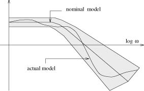
- Suppose P is the nominal model
and K is a controller.
- Nominal Stability (NS): if K stabilizes the nominal P.
- Robust Stability (RS): if K stabilizes every plant in P.
- Nominal Performance (NP): if the performance objectives are satisfied
for the nominal plant P.
- Robust Performance(RP): if the performance objectives are satisfied for
every plant in P.
|
|
3
|
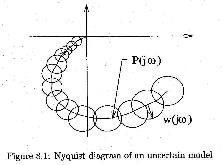
- Example 1: Consider a uncertain transfer function
|
|
4
|
- Another way to bound the frequency response is to treat and as norm
bounded uncertainities; that is,
- P(s,a,b)Î {P0+W1
D1+W2D2 |
||Di||¥ £ 1}
- with P0=P(s,0,0) and
- It is in fact easy to show that
- {P0+W1D1+W2D2 |
||Di||¥ £ 1} = {P0+WD |
||D||¥ £ 1}
- with |W|=|W1|+|W2|.
|
|
5
|
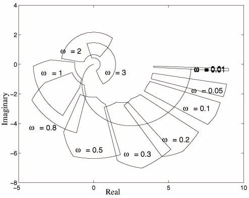
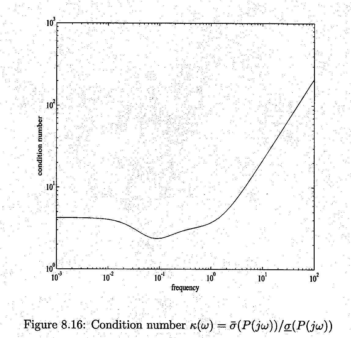
- Example 2: Consider a process control model
- Take the nominal model as
- Then for each frequency, all possible frequency responses are in a box,
as shown in Figure 8.16.
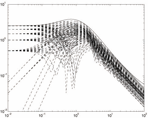
- Da(jw)=G(jw)-G0 (jw)
- To get an additive weighting Wa, use the following Matlab
procedure:
|
|
6
|
- >> mf=ginput(50) % pick 50
points: the first column of mf is the frequency points and the second
column of mf is the corresponding magnitude responses.
- >>magg=vpck(mf(:2),mf(:,1)); % pack them as a varying matrix.
- >> Wa=fitmag(magg); % choose the order of Wa online. A
third-order Wa is sufficient for this example.
- >> [A,B,C,D]=unpck(Wa ) %converting into state-space.
- >> [Z,P,K]=ss2zp(A,B,C,D) % converting into zero/pole/gain form.
|
|
7
|
- We get
- And the frequency response of Wa is also plotted in Figure
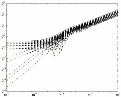
8.17. Similarly, define the multiplicative uncertainty
- and a Wm can be found such that |Dm(jw)|£ |Wm(jw)| as
shown in Figure 8.18. A Wm is given by
|
|
8
|
- Small Gain Theorem: Suppose MÎ (RH¥)pxq . Then the system is well-posed
and internally stable for all D ÎRH¥ with
- (a) ||D||¥ £1/g if and only if ||M||¥ < g ;
- (b) ||D||¥ <1/g if and only if ||M||¥ £ g .
|
|
9
|
- Proof: Assume g = 1. System is stable iff det(I-M D) has no zero in the
closed right-half plane for all D ÎRH¥ and ||D||¥ £1.
- (Ü ) det(I-M D) ¹0 for all D ÎRH¥ and ||D||¥ £1 since
- |l(I-M D) | ³ 1-max| l(M D) | ³ 1- ||M||¥ >0
- (Þ ) Suppose ||M||¥ ³1. There exists a D ÎRH¥ with ||D||¥ £1 such that det(I-M (s)D(s)) has a zero on the imaginary axis, so the
system is unstable. Suppose w Î R+È {¥} is such that
s1(M(jw0 )) ³ 1. Let M(jw0 )= U(jw0 )S(jw0 )V*(jw0 ) be a singular value decomposition
with
- U(jw0 )=[u1,u2,…,up],
V(jw0 )=[v1,v2,…,vp],
- S(jw0 )=diag[s1, s2,…]
|
|
10
|
- We shall construct a D ÎRH¥ such that
D(jw0 )= (1/s1) v1u1*
and ||D||¥ £1. Indeed, for such D(s),
- det(I-M (jw0
)D(jw0 ))=det(I-
U(jw0 )S(jw0 )V(jw0 ) (1/s1) v1u1*
)
- =1- u1* U(jw0 )S(jw0 )V(jw0 )v1
(1/s1)
=0
- and thus the closed-loop system is either not well-posed (if w0 = ¥) or unstable (if w0 Î R+). There
are two different cases:
- (1) w0
= 0 or ¥ :
Then U and V are real matrices. Choose
- D= (1/s1) v1u1*
Î Rqxp
- (2) 0<w0
< ¥ :
write u1 and v1in the following form
- where u1i , v1j Î R are chosen so that qi, fj Î [-p,0).
|
|
11
|
- Choose bi ³0 and aj ³0 so that
- Let
- Then ||D||¥ =1/s1 £1 and D(jw0 )= (1/s1) v1u1* .
|
|
12
|
- The small gain theorem still holds even if D and M are infinite dimensional. This is
summarized as the following corollary.
- Corollary: The following statements are equivalent:
- (i) The system is well-posed and internally stable for all D ÎH¥ with ||D||¥ £1/g .
- (ii) The system is well-posed and internally stable for all D ÎRH¥ with ||D||¥ £1/g .
- (iii) The system is well-posed and internally stable for all D ÎRqxp with ||D|| £1/g .
- (iv) ||M||¥ £ g
- It can be shown that the small gain
condition is sufficient to guarantee internal stability even if D is a nonlinear and
time varying “stable” operator with an appropriately defined stability
notion, see Desoer and Vidyasagar [1975].
|
|
13
|
- Define
- So=(I+PK)-1, To=PK(I+PK)-1
Si=(I+KP)-1, Ti=KP(I+KP)-1
- Let P={P+W1 DW2 : D Î RH¥ }
and let K stabilize P. Then the
closed-loop system is well-posed and internally stable for all ||D||¥ <1 if
and only if ||W2KSoW1 ||¥ £ 1.
|
|
14
|
- Define
- So=(I+PK)-1, To=PK(I+PK)-1
Si=(I+KP)-1, Ti=KP(I+KP)-1
- Let P={(I+W1 DW2)P: D Î RH¥ }
and let K stabilize P. Then the
closed-loop system is well-posed and internally stable for all ||D||¥ <1 if
and only if ||W2ToW1 ||¥ £ 1.
|
|
15
|
- Let be stable left
coprime factorization and let K stabilize P. Suppose
- with Then
the closed-loop system is well-posed and internally stable for all ||D||¥ <1 if
and only if
|
|
16
|
|
|
17
|
|
|
18
|
- Consider a feedback system with uncertain plant PD ,
the weighted sensitivity function is defined as the transfer function
from d to e:
- Suppose our performance
objective is
- ||Ted||¥ =sup{||d||2 £1} ||e||2 £1
- Suppose PD Î {(I+DW2)P: D Î RH¥ , ||D||¥ <1 } and K stabilizes P. Then the robust
performance is guaranteed if
|
|
19
|
- Suppose PD Î {P(I+wD): D Î RH¥ , ||D||¥ <1 } and
K stabilizes P.
- robust stability:
- ||wTi||¥ £1
- nominal performance:
- ||WeSo||¥ £1.
- robust performance is guaranteed if
|
|
20
|
- Covering Uncertainty:
- since
|
|
21
|
|
|
22
|
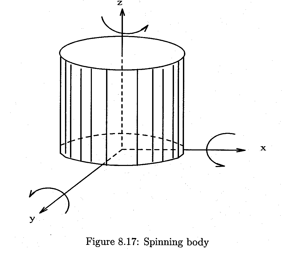
- Spinning body with constant velocity in the z direction.
|
|
23
|
- Each loop has the open-loop transfer function as 1/s so each loop has
phase margin fmax=-fmin=90o
and gain margin kmax=0, kmin=¥
- Suppose one loop transfer function is
perturbed
- Denote z(s)/w(s)=-T11(s) = -1/(s+1). Then the maximum
allowable perturbation is ||d||¥ <1/||T11(s)||¥ =1, which
is independent of a.
- However, if both loops are perturbed at the same time, then the maximum
allowable perturbation is much smaller, as shown below
- The system is robustly stable for every such D iff
|
|
24
|
|
|
25
|
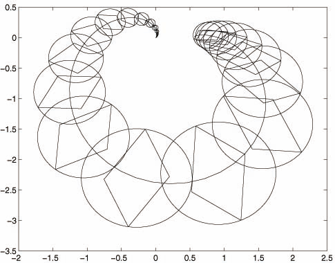
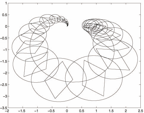
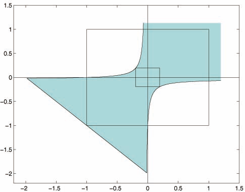
- In particular, consider
- Then the closed-loop system is stable for every such D iff
- has no zero in the closed right-half plane.
- Hence the stability region is given by
- 2+ d11+
d22 >0, 1+d11+d22+(1+a2)d11d22>0
- The system is unstable with
- d11 =-d22 = (1+a2)-1/2
|

 Notes
Notes